
What makes data-based questions difficult?

In a chapter exercise, the question often tells you which principle to use. A data-based task asks you to make that choice. A measured gradient might represent a spring constant, its reciprocal or a quantity that still needs a unit conversion. An apparently straight graph might support a linear model without supporting direct proportionality.

The current IB Physics course identifies uncertainty processing, graph interpretation and experimental reasoning among its required skills. Paper 1B gives these skills a dedicated data-based setting. Check the official Physics guide for your course requirements.

This article contains seven original teaching problems, not official examination questions or predictions. The numerical uncertainty exercises explicitly use simple conservative propagation: add absolute uncertainties for addition or subtraction, and add fractional uncertainties for multiplication or division. Follow any different convention stated in an actual question.

Before you calculate: identify the measured quantities, the quantity you need, the relationship between them and the units on every axis. Those four decisions prevent many avoidable mistakes.

Try the seven traps before opening the solutions

Choose an answer, but also write one sentence defending it. A correct choice reached by an unreliable method still needs review. Use the hints only after making an independent attempt; the solutions explain the reasoning and the limits of each conclusion.

Try it here

Seven original Paper 1B skill checks

Choose one answer per problem. All measurement models and uncertainty conventions needed are stated in the questions.

Question 01 · Repeated timing1. Dividing the value but forgetting the uncertainty. Three measurements for 20 oscillations are 32.4 s, 32.6 s and 32.8 s. Use the mean time and half the range as its uncertainty; ignore other uncertainty sources. What is the period?
Need a hint?
The period and its absolute uncertainty are both obtained by dividing by the exact count of 20.
Worked solution

The mean time is (32.4 + 32.6 + 32.8)/3 = 32.6 s. Half the range is (32.8 − 32.4)/2 = 0.2 s. Therefore T = 32.6/20 = 1.63 s and ΔT = 0.2/20 = 0.01 s. The result is (1.63 ± 0.01) s.

The count of 20 oscillations is treated as exact. Dividing only the central value leaves an uncertainty for the wrong quantity. Dividing the uncertainty twice would also be wrong. This simple exercise illustrates repeatability; in a real timing experiment, reaction time or calibration effects may require additional treatment.

Question 02 · Uncertainty in a difference2. Subtracting uncertainties. The two ends of a small displacement are read as (12.4 ± 0.1) cm and (18.1 ± 0.1) cm. Treat the reading uncertainties as separate bounds and use conservative propagation. What is the displacement?
Need a hint?
Find the largest possible separation and the smallest possible separation.
Worked solution

The central displacement is 18.1 − 12.4 = 5.7 cm. The largest possible value is 18.2 − 12.3 = 5.9 cm; the smallest is 18.0 − 12.5 = 5.5 cm. Thus the conservative uncertainty is 0.2 cm and the result is (5.7 ± 0.2) cm.

For subtraction, the numerical readings subtract while their separate absolute uncertainty bounds add. This conclusion uses the stated model. A common calibration offset affecting both readings equally could cancel in a difference; you should not assume that correlation unless the experiment gives a reason.

Question 03 · Powers and fractional uncertainty3. Forgetting the power. A pendulum estimate uses g = 4π²L/T², with L = (0.800 ± 0.004) m and T = (1.80 ± 0.02) s. Treat 4π² as exact. Using conservative fractional propagation, what is the percentage uncertainty in g, to two significant figures?
Need a hint?
The fractional uncertainty in T² is twice the fractional uncertainty in T.
Worked solution

For g proportional to L/T², Δg/g ≈ ΔL/L + 2ΔT/T. Substitution gives 0.004/0.800 + 2(0.02/1.80) = 0.027222… . The percentage uncertainty is therefore 2.7%.

The central estimate is g = 4π²(0.800)/(1.80)² ≈ 9.75 m s−2, with absolute uncertainty about 0.27 m s−2. A one-significant-figure uncertainty presentation would be (9.7 ± 0.3) m s−2. Carry guard digits during the calculation. Adding 0.004 and 0.02 directly would combine quantities with different units and has no useful meaning.

Question 04 · Axes, units and inverse gradients4. Reading the gradient as the wrong constant. A graph has extension x in cm vertically and force F in N horizontally. Two points on the fitted line are (1.0 N, 1.35 cm) and (4.0 N, 4.35 cm). If x = F/k + x₀, what is k?
Need a hint?
First find Δx/ΔF in metres per newton. It equals 1/k.
Worked solution

The gradient is (4.35 − 1.35)/(4.0 − 1.0) = 1.00 cm N−1 = 0.0100 m N−1. Comparing x = F/k + x₀ with y = mx + c shows that the gradient is 1/k. Hence k = 1/0.0100 = 100 N m−1.

A useful dimensional check is that spring stiffness measures force per extension. The plotted gradient measures extension per force, so an inverse is required. The nonzero intercept does not alter this gradient calculation; it changes the interpretation of the zero-load reading.

Question 05 · Linear versus proportional5. Treating every straight line as direct proportion. Extension data are consistent with x/cm = F/N + 0.35 over the tested range. Which conclusion is justified by that relationship alone?
Need a hint?
Direct proportionality needs a zero intercept; identifying the cause of an intercept needs additional evidence.
Worked solution

The supported statement is a linear relationship with a positive intercept. Direct proportionality would require x = cF, so the graph would pass through the origin. A nonzero intercept could result from an offset, an initial extension or the definition of the measured quantity.

The graph does not identify a particular faulty instrument. Nor does a fit over a limited range establish behaviour outside that range. A strong experimental answer says what the data support and proposes a further measurement when several explanations remain possible.

Question 06 · Logarithmic graphs6. Reading a log-gradient as an ordinary rate. Intensity obeys I = A/r² for positive r. A graph plots log₁₀(I/I₀) vertically against log₁₀(r/r₀) horizontally, with fixed positive reference values I₀ and r₀. What is its gradient?
Need a hint?
Rewrite I/I₀ using the dimensionless ratio r/r₀, then take logarithms.
Worked solution

Write I/I₀ = [A/(I₀r₀²)](r/r₀)−2. Taking base-10 logarithms gives log₁₀(I/I₀) = log₁₀[A/(I₀r₀²)] − 2log₁₀(r/r₀). The gradient is therefore −2.

The slope gives the exponent in the power relationship; it is not dI/dr. The reference quantities keep the logarithm arguments dimensionless and only affect the intercept. As a quick physical check, doubling r quarters I, consistent with an inverse-square dependence.

Question 07 · Gradient bounds7. Confusing the full range with an uncertainty. After checking every uncertainty bar, the smallest and largest acceptable gradients are 0.84 and 1.16 m s⁻². Use half the range to estimate the gradient uncertainty. What is that uncertainty?
Need a hint?
The total width between the two limiting gradients covers both sides of the central estimate.
Worked solution

The uncertainty estimate is (1.16 − 0.84)/2 = 0.16 m s−2. The midpoint is 1.00 m s−2, so a corresponding result is (1.00 ± 0.16) m s−2.

The limiting lines must be compatible with all the stated bars, not just the first and last measurements. A steep line that misses a middle bar is not an acceptable bound. This geometric range estimate is also different from a statistical standard error; use the method the task specifies.

This is a seven-skill practice check. It is not an IB grade estimate or a prediction of performance on a full examination.

A straight line can still miss the origin

The example below plots measured extension against applied force. The bars show ±0.2 cm uncertainty in each extension; force uncertainty is negligible for this exercise. The fitted relationship is x/cm = F/N + 0.35.
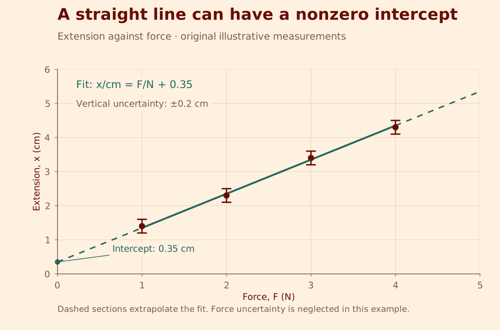
Extension–force data with ±0.2 cm uncertainty bars and a fitted intercept of 0.35 cm.
Original illustrative data. Vertical bars show ±0.2 cm; the dashed segment extrapolates the fitted line. A straight line need not pass through the origin.

A useful answer distinguishes three statements. The data are consistent with the displayed straight line. The fitted intercept is positive. A zero offset is one possible explanation, but the graph alone does not establish its cause. You would need a zero-load reading, an instrument check or more information about how extension was defined.

To test a proposed line, inspect every uncertainty bar. A line through the origin that reaches the first bar needs a numerical slope of at least 1.2. A line through the origin that reaches the last bar needs a slope no greater than 1.125. Those requirements conflict, so no single origin-passing line crosses all four bars under the stated assumptions. That is stronger reasoning than saying the points merely “look shifted”.

Turn your working into a scientific answer

Use a short chain: quantity → calculation → units → interpretation. For a gradient, state the two coordinates chosen from the fitted line, calculate the change in the vertical quantity divided by the change in the horizontal quantity, and interpret the units. Use a large triangle where possible; two adjacent measured points unnecessarily magnify reading uncertainty.

For a comparison, state the values or intervals being compared. “The values agree” is incomplete when the question provides uncertainties. “The accepted value lies inside the experimental interval, so these results are compatible at the stated uncertainty” explains the actual test. Compatibility does not prove the model, and non-overlap may reflect an underestimated uncertainty as well as a wrong model.

For an improvement, connect the change to a mechanism. “Repeat it” is weak when a balance has a zero error. Checking the empty balance and applying the correction addresses that offset. Repeating measurements can reveal scatter; it does not automatically remove a calibration problem.

Try it here

Before you move on

Check each item only when you can explain it using one of the examples above.

Your checked items are stored only on this device when browser storage is available.

Completing a checklist records your review; it does not certify mastery.

A focused 30-minute practice session

Study suggestion: spend 10 minutes attempting a small set without notes, 10 minutes reviewing the first incorrect decision in each solution, and 10 minutes solving a fresh version. Change a unit, swap the axes or change a squared variable to an unsquared one. If your method survives that change, you are learning the underlying skill.

Keep a brief error log with three columns: the decision, the evidence you overlooked and the rule you will apply next time. Write “I treated cm/N as N/m” rather than “careless mistake”. A precise diagnosis gives you a precise next task.

When you can solve the mini-problems, combine them with the physics of an unfamiliar context. Explain why the measured variables should be related, then process the data. Topic knowledge and data handling become more useful when you practise them together.

Before you go

Common questions

Is Paper 1B only about uncertainty calculations?
No. Uncertainty is one part of data-based reasoning. You may also need physics knowledge, graphs, units, experimental design and a justified interpretation of evidence.
Should I use measured points or the fitted line for a gradient?
When asked for the gradient of a fitted line, use well-separated points on that line. They do not have to be original measurements. State the coordinates and units clearly.
Does repeating a measurement remove a systematic error?
Repetition can help you investigate scatter and improve a mean under a suitable model. A persistent calibration or zero error needs a relevant check or correction.
Can older data-analysis questions still help?
They can develop overlapping skills. Check their content and assessment demands against your current course rather than treating an old paper as an exact current-format mock.
Are these official IB questions or mark schemes?
No. The questions, explanations and checking tools here are original teaching resources by Thriving Scholars. The official guide is linked for the course requirements.

Sources & further reading

Official rules and programme details can change. Use the linked source for your exact course, competition or examination session.

  1. IB Physics guide — first assessment 2025Current data-processing, graphing and assessment skills; original exercises are not reproduced from this guide.
  2. IB Physics course overviewCurrent subject context and the role of data analysis.